1. What is the difference between shallow copy and deep copy in System Verilog? Explain with an example.

Shallow Copy:
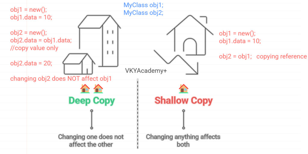
Copies only the reference to an object, not the actual object. Changes to one will affect the other.

Deep Copy:
Copies the entire object and its contents, creating an independent duplicate. Changes to one will not affect the other.

Shallow Copy: Example

class MyClass;
  int data;
endclass

module test;
  initial begin
    MyClass obj1; 
    MyClass obj2;

    obj1 = new();  // first create object
    obj1.data = 10;

    obj2 = obj1;   // shallow copy (copying reference)

    obj2.data = 20; // changing obj2 also changes obj1

    $display("obj1.data = %0d", obj1.data); // Output: 20

    $display("obj2.data = %0d", obj2.data); // Output: 20
  end
endmodule

/*==================
//Output:
//==================
obj1.data = 20

obj2.data = 20
================== */

Explanation :
In this code, a class MyClass with an integer variable data is defined. Inside the test module, two object handles obj1 and obj2 are declared. obj1 is created using new() and assigned the value 10. Then, obj2 is made to point to the same object as obj1, meaning both obj1 and obj2 now reference the same memory location — this is called a shallow copy. When obj2.data is changed to 20, it also changes obj1.data because both are sharing the same object. Therefore, the output shows both obj1.data and obj2.data as 20, confirming that shallow copy only copies the reference, not the actual data.

Deep Copy : Example

class MyClass;
  int data;
endclass

module test;
  initial begin
    MyClass obj1;
    MyClass obj2;

    obj1 = new();
    obj1.data = 10;

    obj2 = new();
    obj2.data = obj1.data; // deep copy (copy value only)

    obj2.data = 20; // changing obj2 does NOT affect obj1

    $display("obj1.data = %0d", obj1.data); // Output: 10

    $display("obj2.data = %0d", obj2.data); // Output: 20
  end
endmodule


/*==================
Output:
==================
obj1.data = 10

obj2.data = 20
==================*/

Explanation :
In this code, a class MyClass with an integer variable data is defined. Inside the test module, two object handles obj1 and obj2 are declared. obj1 is created using new() and its data is set to 10. Then a completely new object obj2 is also created separately using new(), and its data is manually assigned the value of obj1.data, copying just the data and not the object reference. Since obj1 and obj2 now point to two different memory locations, when obj2.data is later changed to 20, it does not affect obj1.data. As a result, the output shows obj1.data = 10 and obj2.data = 20, demonstrating that deep copy creates two independent objects.

Shallow Copy → Two people living in the same house 🏠 → Changing anything affects both.

Deep Copy → Two people living in different houses 🏠🏠 → Changing one does not affect the other.

2. Write a System Verilog code to generate Fibonacci series.

What is a Fibonacci Series?
The Fibonacci series is a special sequence of numbers where each number is the sum of the two numbers immediately before it. It typically starts with 0 and 1, and continues as 0, 1, 1, 2, 3, 5, 8, 13, and so on. Each number in the series naturally grows based on the pattern of addition, and the sequence often appears in various patterns in nature, mathematics, and computer science problems. The Fibonacci series is valued for its simplicity and its surprising connections to real-world phenomena.

module fibonacci;

  int a = 0, b = 1, c, n = 10; // 'n' is the number of terms

  initial begin
    $display("Fibonacci Series:");

    $display("%0d", a);

    $display("%0d", b);

    for (int i = 2; i < n; i++) begin
      c = a + b;

      $display("%0d", c);

      a = b;
      b = c;
    end
  end
endmodule
/*
======================
Output:
======================
Fibonacci Series:
0
1
1
2
3
5
8
13
21
34
===================== */

Explanation :
In this SystemVerilog code, we generate a Fibonacci series using a very straightforward approach. We start by initializing the first two numbers of the series, a = 0 and b = 1. Inside the initial block, we first display these two starting numbers. Then, using a simple for loop, we calculate each next number c as the sum of the previous two (a + b). After calculating and displaying c, we update a and b so that the next iteration can continue building the sequence. This process is repeated until we generate the desired number of terms (n = 10 in this case). The code uses no complex functions, keeping it clear and beginner-friendly.

3 . Write a System Verilog code to generate prime numbers from 1 to 50.

What is a prime number?
A prime number is a natural number greater than 1 that can only be divided exactly by 1 and itself. In other words, a prime number has no divisors other than 1 and the number itself. Examples of prime numbers are 2, 3, 5, 7, 11, 13, and so on.

module prime_numbers;

  int n = 20; // Define the range (1 to n)

  int num, i;

  bit is_prime;

  initial begin

    $display("Prime numbers between 1 and %0d are:", n);
    
    // Iterate over all numbers from 2 to n
    for (num = 2; num <= n; num++) begin

      is_prime = 1;  // Assume 'num' is prime initially
      
      // Check divisibility from 2 to sqrt(num)

      for (i = 2; i * i <= num; i++) begin

        if (num % i == 0) begin

          is_prime = 0;  // num is not prime

          break;  // No need to check further

        end

      end

      // If prime, display the number

      if (is_prime)

        $display("%0d", num);

    end

  end

endmodule


/*
================================
Output:
===============================
Prime numbers between 1 and 20 are:
2
3
5
7
11
13
17
19
===============================
*/

Explanation :
This SystemVerilog code finds and prints all prime numbers between 1 and a given number n.
For each number from 2 to n, it assumes the number is prime, then checks if it is divisible by any number from 2 up to the square root of that number.

• If a divisor is found, it marks the number as not prime.
• If no divisors are found, it prints the number as a prime.

The optimization i * i <= num ensures that we only check divisibility up to the square root, making the code faster and more accurate.

Mistakes We Must Avoid (Important Learning)

1. Incomplete Divisibility Check:
   • Checking divisibility only up to num/2 or smaller ranges can miss detecting factors for some numbers, leading to wrong results.
   • Always check up to sqrt(num) (or full range 2 to num-1 if sqrt is confusing).
2. Wrong Loop Bounds:
   • If you wrongly set loop conditions like i <= num/2 without understanding why, it can make the program behave incorrectly.
3. Skipping Early Exit (break):
   • Once a number is found divisible, immediately break the loop to save unnecessary checks.
4. Testing Before Assuming:
   • Always test with a few numbers manually (like 5, 7, 11, etc.) to ensure the prime-checking logic is correct.

❌ Incorrect Divisibility Range:
Checking up to num-1 instead of sqrt(num) wastes time and may miss correct results.

❌ Missing Break Condition:
Forgetting to break after finding a divisor leads to unnecessary extra checks.

❌ Not Testing with Sample Numbers:
Always manually test edge cases like 5, 7, 11 to catch mistakes early.

How Prime Number Checking Works :

The below table helps in understanding and makes the coding easier for us in prime number checking. Suppose we want to check if 17 is prime:

Divisor i	Condition i * i <= 17	Check 17 % i	Result
2	4 <= 17 ✔️	17 % 2 = 1	Not Divisible
3	9 <= 17 ✔️	17 % 3 = 2	Not Divisible
4	16 <= 17 ✔️	17 % 4 = 1	Not Divisible
5	25 <= 17 ❌ (Stop)

class PrimeGenerator;
  rand int number;  // Random number to check for primality
  int limit;        // Upper limit (N)

  // Constructor
  function new(int n);
    limit = n;
  endfunction

  // Constraint: number must be between 2 and limit
  constraint range_c { number inside {[2:limit]}; }

  // Function to check if a number is prime
  function bit is_prime(int num);
    int i;
    for (i = 2; i * i <= num; i++) begin
      if (num % i == 0)
        return 0;
    end
    return 1;
  endfunction
endclass

module prime_class_example;
  PrimeGenerator pg;
  int num;

  initial begin
    int N = 20;
    pg = new(N);

    $display("Prime numbers between 1 and %0d are:", N);

    for (num = 2; num <= N; num++) begin
      if (pg.is_prime(num))
        $display("%0d", num);
    end
  end
endmodule

/*
===============================
Output:
==============================
Prime numbers between 1 and 20 are:
2
3
5
7
11
13
17
19
============================
*/

In the above code the number is randomized inside 2 to limit using constraint.

randomize_prime() is a smart method that:

• Randomizes a number
• Checks if it's a prime using is_prime()
• If not prime, it keeps randomizing until it gets a prime

So, when you run it, you’ll get random prime numbers!

Feature	Benefit
Constraints	Limit random numbers between [2:N] easily
Functions	Perform prime checking efficiently
Randomization	Get different prime numbers every simulation
Cleaner design	Separation of concerns (constraint vs checking logic)

One question always arise in the mind of every design and verification engineer , Why Class-Based Architecture is Better than Simple Static/Module-Based Coding?

Aspect	Static/Module-Based Code	Class-Based Code
Flexibility	Rigid and hard to extend	Highly flexible and reusable
Data Encapsulation	Everything exposed globally	Data + functionality hidden inside objects
Reusability	Code often duplicated	Class objects reused across projects
Maintainability	Harder to debug and modify	Easy to debug, modular, and organized
Scalability	Becomes messy as size grows	Handles complex systems easily
Advanced Features	No support for inheritance, polymorphism	Full support — can build powerful hierarchies
Real-World Modeling	Not natural for real systems	Very close to modeling real hardware behaviors
Testbench/Verification	Difficult to randomize	Powerful randomization + constraints built-in

In Real-Time / Hardware Design Purpose:

✔️ 1. Modeling Real-World Entities

When designing hardware blocks (like ALUs, Memory Controllers, FIFOs), they have properties (data) and behaviors (methods).
👉 Classes naturally represent them like real-world objects.

Example:

• ALU has inputs, outputs, and operations → a class can model all that neatly.

---

✔️ 2. Better for Testbench and Verification

When verifying hardware (in UVM or other methodologies),

• We create random stimulus.
• We create scoreboards, drivers, monitors.
• All these are beautifully modeled as classes.

👉 Imagine if everything were static — impossible to scale and extend!

---

✔️ 3. Reuse Across Projects

Classes can be written once and reused across multiple projects or IPs.
Example:

• A Packet class for Ethernet can be reused in WiFi, PCIe, etc.
• No need to write again and again.

---

✔️ 4. Constraints and Randomization

Classes allow constrained random stimulus easily, which is critical in coverage-driven verification.
Without classes, random generation would be painful and manual.

Lets understand with the help of DDR memory example:

• Imagine you are building a DDR Memory Controller.
• You need to generate 1000s of random read/write transactions.
• You need to monitor data consistency and timing violations.

Without classes ➔ total mess. ❌
With classes ➔ clean architecture:

• Transaction class
• Monitor class
• Scoreboard class
• Driver class
• and more.

Classes make big projects manageable and future-proof.

4 . Given an array with elements {50, 10, 0, 40, 20, 30}, write a System Verilog code to print the array in descending order.

module sort_descending;
  int arr[6] = '{50, 10, 0, 40, 20, 30};
  int i, j, temp;

  initial begin
    // Sorting using simple nested loops
    for (i = 0; i < 6; i++) begin
      for (j = i+1; j < 6; j++) begin
        if (arr[i] < arr[j]) begin
          temp = arr[i];
          arr[i] = arr[j];
          arr[j] = temp;
        end
      end
    end

    // Printing the sorted array
    $display("Array in Descending Order:");
    foreach (arr[k])
      $display("%0d", arr[k]);
  end
endmodule

/*
======================
Output:
======================
Array in Descending Order:
50
40
30
20
10
0
======================
*/

The outer loop (i) picks each element one by one.

The inner loop (j) checks all elements after i.

If any element at j is greater than the element at i, we swap them.

This way, the largest elements "bubble up" to the beginning of the array.

Finally, the array gets printed from highest to lowest value.

Class based coding approach:

class ArraySorter;
  int arr[];

  // Constructor to initialize the array
  function new(int input_array[]);
    arr = new[input_array.size()];
    arr = input_array;
  endfunction

  // Method to sort in descending order
  function void sort_descending();
    int i, j, temp;
    for (i = 0; i < arr.size(); i++) begin
      for (j = i+1; j < arr.size(); j++) begin
        if (arr[i] < arr[j]) begin
          temp   = arr[i];
          arr[i] = arr[j];
          arr[j] = temp;
        end
      end
    end
  endfunction

  // Method to display the array
  function void display_array(string msg);
    $display("%s %p", msg, arr);
  endfunction
endclass

module sort_descending_class;
  int input_arr[] = '{50, 10, 0, 40, 20, 30};
  ArraySorter sorter;

  initial begin
    sorter = new(input_arr);          // Create object and initialize array
    sorter.display_array("Original Array:"); 
    sorter.sort_descending();         // Sort the array
    sorter.display_array("Sorted Array (Descending):");
  end
endmodule


/*
================================
Output:
================================
Original Array: '{50, 10, 0, 40, 20, 30}
Sorted Array (Descending): '{50, 40, 30, 20, 10, 0}
================================
*/

Aspect	Using Task	Using Class
Reusability	Sort any array by calling the task	Create multiple objects for different arrays
Modularity	Separates sorting logic from main flow	Data + sorting logic packaged together
Encapsulation	Not applicable	Fully encapsulated (clean & maintainable)
Extensibility	Limited (need to modify task for changes)	Easy to add new features (e.g., ascending sort)
Best Use Cases	Small programs or testbenches	Larger projects, scalable designs, or verification environments

5. If functional coverage is 100% and code coverage is 50%, is it acceptable to close the project? What about the reverse scenario?

Answer:

If Functional Coverage = 100% and Code Coverage = 50%:

• Not acceptable to close the project!
• Reason: Even though all planned features (functional intents) are tested (100%), only 50% of the code is actually exercised during simulation.
• ➡️ This hints that half of the code might be untested, dead, redundant, or unreachable.
• There could be hidden bugs in the unused code paths which might create serious issues in silicon.
• Action: Analyze uncovered code, check for missing test scenarios, improve testbench, or clean up dead code if not needed.

---

If Functional Coverage = 50% and Code Coverage = 100%:

Action: Add more functional tests, cover corner cases, boundary conditions, and unexpected scenarios until functional coverage approaches 100%.

Also not acceptable to close the project!

Reason: Although the simulator touched every line and branch of the code (100%), only half of the functional features or corner cases are properly tested.

➡️ This means the tests are very basic or shallow — they just "run through" the code without validating the real design behavior thoroughly.

Scenario	Decision	Reason
Functional 100%, Code 50%	❌ Don't close	Some code is not tested, risk of bugs
Functional 50%, Code 100%	❌ Don't close	Features are not properly validated

👉 Both Functional and Code Coverage should be reasonably high (close to 100%) before confidently closing the project!
(Some companies set thresholds like 90%+ for both, depending on the risk level.)

6. What is the difference between issuing a write and precharge at the same time versus issuing a write followed by precharge? Which one is logically correct? If both have some significance explain ?

Answer:

Scenario	Explanation
Issuing WRITE and PRECHARGE at the same time	Here, the WRITE command is sent to the memory along with a flag/request that tells the memory: "After this WRITE is complete, immediately precharge (close) the row." It’s like writing something in a book and slamming it shut right after you're done.
Issuing WRITE first and PRECHARGE later	In this case, first a WRITE command is issued and after some delay or after confirming something, a PRECHARGE command is sent separately. This gives you manual control to decide when to close the row — maybe after doing more reads or writes to the same row.

✅ Which one is logically correct?

Both are logically correct — but which one you should use depends on the situation:

Condition	Preferred Style
If you are done with that row (no more read/writes needed)	WRITE with AUTO-PRECHARGE (together)
If you want to access (read/write) more data from the same row	WRITE first, then PRECHARGE manually later

Real-World Significance:

• Write + Auto-Precharge (together):
  • Faster if you know you don’t need anything else from that row.
  • Reduces controller complexity because memory will auto-handle precharge timing.
  • Useful for random access patterns.
• Write then Precharge separately (manual control):
  • More flexible if you are doing burst reads/writes from the same open row.
  • Improves memory efficiency (row hit advantage) because opening and closing a row costs extra time.
  • Used in optimized memory controllers like in DDRs for high throughput.

7. What is the difference between pre-silicon and post-silicon validation? What types of faults cannot be rectified in post-silicon and must be verified during pre-silicon?

Answer:

Property	Pre-Silicon Validation	Post-Silicon Validation	Effect if Missed
When it Happens	Before chip fabrication (simulation, emulation, formal methods)	After actual silicon is manufactured	Pre-silicon mistakes cause expensive re-spins
Environment	Virtual environment (using models, RTL simulation, formal verification, emulation)	Real physical hardware (using logic analyzers, testers, boards)	Pre-silicon is faster, more flexible to fix
Goal	Catch logic/design bugs, functional correctness, timing, and protocol violations	Catch manufacturing defects, real-world issues like power, performance, thermal	Pre-silicon misses can lead to hardware bugs that are impossible to fix later
Faults Typically Detected	Logical/functional bugs, design errors, timing violations, deadlocks, protocol violations	Signal integrity issues, marginal timing, power consumption problems, rare corner cases	Logical bugs missed in pre-silicon cannot be easily fixed post-silicon
Faults that Must be Verified Pre-Silicon	Protocol violations, functional mismatches, deadlocks, design feature issues	—	These are embedded into chip logic — post-silicon can't repair easily
Flexibility to Fix	High (can change RTL/design easily)	Very low (limited to workarounds or masks; major re-spin needed otherwise)	Fixing issues in post-silicon is very expensive and delays product
Cost of Fixing Bugs	Low (just recompile RTL or re-simulate)	Very High (new silicon tapeout, huge cost and delay)	Catching critical bugs pre-silicon saves millions 💰
Examples	Missing a signal handshake, wrong ALU operation, bad reset logic, incorrect cache coherence	Unexpected EMI issues, timing due to process variation, rare hardware hangs under extreme thermal stress	Missing functional issues pre-silicon means chip re-design required

8. Explain the concept of polymorphism in System Verilog with a simple example.

Answer :

What is Polymorphism in SystemVerilog?

• Polymorphism means "same function behaves differently for different classes".
• It allows us to call a method from a base class but execute the derived class’s version of that method at runtime.
• In short: One interface, multiple behaviors.

class Animal;
  // Virtual method
  virtual function void sound();
    $display("Animal makes a sound");
  endfunction
endclass

class Dog extends Animal;
  // Override method
  function void sound();
    $display("Dog barks");
  endfunction
endclass

class Cat extends Animal;
  // Override method
  function void sound();
    $display("Cat meows");
  endfunction
endclass

module test;
  initial begin
    Animal a;        // Base class handle
    Dog d = new();   // Derived class object
    Cat c = new();   // Derived class object

    // Polymorphism in action
    a = d; 
    a.sound(); // Output: Dog barks

    a = c;
    a.sound(); // Output: Cat meows
  end
endmodule

/*
=============
Output:
=============
Dog barks
Cat meows
=============
*/

• Animal is the base class.
• Dog and Cat are child classes and override the sound() method.
• When we assign a = d and a.sound(), Dog's version is called.
• When we assign a = c and a.sound(), Cat's version is called.

Even though we use a base class handle (a), different versions of sound() run depending on the object (Dog or Cat) it points to.
That is polymorphism — one name, many forms!

Imagine you have a universal remote control (base class). This remote can control multiple devices like a TV, Air Conditioner, and Fan (derived classes). Even though the same remote (the base class) is used to control all the devices, each device responds in a different way.

"Just like a universal remote control works with multiple devices, polymorphism in SystemVerilog allows the same method name to invoke different behaviors depending on the object it’s controlling. One interface, many actions!"

9. What is the difference between ATPG and MBIST?

Answer:

Both ATPG and MBIST are crucial techniques used in VLSI (Very-Large-Scale Integration) design, specifically in testing and ensuring the reliability of semiconductor devices. Though both serve the purpose of detecting faults, they are designed for different scenarios and can't always be used interchangeably.

---

Real-time Project Example:

Imagine you're working on a complex SoC (System on Chip) that includes a CPU, memory modules, and other logic units.

1. ATPG - Automatic Test Pattern Generation

• Purpose: ATPG is primarily used to generate test patterns to validate the logic of the chip. This is essential for catching faults like stuck-at faults, bridging faults, and delay faults in the combinational logic of the chip.
• Use Case in a Project:
  • Let’s say your project involves testing the CPU core for logical errors. You’ll use ATPG to generate input vectors that cover various test scenarios for the logic gates inside the CPU (AND, OR, XOR, etc.).
  • For example: If a gate in the CPU has a fault where it always stays stuck at 1 (stuck-at fault), ATPG would generate a test vector to identify this failure by simulating the logic behavior under various conditions.
  • Key Features:
    • ATPG focuses on functional logic testing.
    • It works at the gate-level and is typically applied to test non-memory logic.

2. MBIST - Memory Built-In Self-Test

• Purpose: MBIST is specifically designed for testing memory units (like SRAM, DRAM, or Flash). It checks for faults like stuck bits, open rows/columns, and other memory-specific issues.
• Use Case in a Project:
  • Your SoC might have an SRAM or DRAM block as part of its memory subsystem. For example, an embedded controller might be running an MBIST controller that tests the SRAM module.
  • For example: If there's a bit in the memory that is always stuck (i.e., it always reads as 0 or 1), MBIST would generate patterns to detect such faults, helping ensure that the memory cells are functioning correctly before the chip is shipped.
  • Key Features:
    • MBIST focuses on memory testing only.
    • It works at the memory cell level and is applied to ensure memory integrity.

Property	ATPG	MBIST
Purpose	Tests the logic (gates, combinational)	Tests memory (SRAM, DRAM, Flash, etc.)
Target	Logic and circuits (non-memory)	Memory subsystems (SRAM, DRAM)
Method	Generates test vectors for fault detection in logic	Built-in hardware test controllers to test memory
Faults Detected	Stuck-at faults, bridging faults, logic errors	Memory cell faults, stuck bits, read/write errors
Application	Used to test CPUs, ALUs, etc.	Used to test memory modules like RAM and cache
Technology	Typically involves functional simulation	Involves hardware controllers integrated into the chip
Test Methodology	Involves external ATPG tools	Self-test performed by the chip itself via MBIST controllers

Solution to Embedded Engineer Interview Questions:Part-1